This is a utility function to extract the underlying data from
a gt table. You can use it with a saved gt table, in the pipe (%>%)
or even within most other gt functions (eg tab_style()). It defaults to
returning the column indicated as a vector, so that you can work with the
values. Typically this is used with logical statements to affect one column
based on the values in that specified secondary column.
Alternatively, you can extract the entire ordered data according to the
internal index as a tibble. This allows for even more complex steps
based on multiple indices.
See also
Other Utilities:
add_text_img(),
fa_icon_repeat(),
fmt_pad_num(),
fmt_pct_extra(),
fmt_symbol_first(),
generate_df(),
gt_add_divider(),
gt_badge(),
gt_double_table(),
gt_duplicate_column(),
gt_fa_rank_change(),
gt_fa_rating(),
gt_highlight_cols(),
gt_highlight_rows(),
gt_img_border(),
gt_img_circle(),
gt_img_multi_rows(),
gt_img_rows(),
gt_merge_stack(),
gt_merge_stack_color(),
gt_two_column_layout(),
gtsave_extra(),
img_header(),
pad_fn(),
tab_style_by_grp()
Examples
library(gt)
# This is a key step, as gt will create the row groups
# based on first observation of the unique row items
# this sampling will return a row-group order for cyl of 6,4,8
set.seed(1234)
sliced_data <- mtcars %>%
dplyr::group_by(cyl) %>%
dplyr::slice_head(n = 3) %>%
dplyr::ungroup() %>%
# randomize the order
dplyr::slice_sample(n = 9)
# not in "order" yet
sliced_data$cyl
#> [1] 6 6 6 4 8 4 8 8 4
# But unique order of 6,4,8
unique(sliced_data$cyl)
#> [1] 6 4 8
# creating a standalone basic table
test_tab <- sliced_data %>%
gt(groupname_col = "cyl")
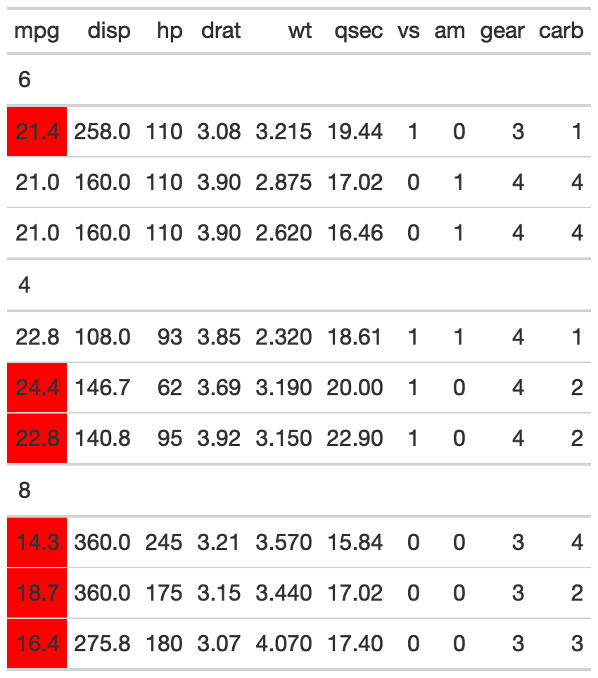
# can style a specific column based on the contents of another column
tab_out_styled <- test_tab %>%
tab_style(
locations = cells_body(mpg, rows = gt_index(., am) == 0),
style = cell_fill("red")
)
# OR can extract the underlying data in the "correct order"
# according to the internal gt structure, ie arranged by group
# by cylinder, 6,4,8
gt_index(test_tab, mpg, as_vector = FALSE)
#> # A tibble: 9 × 11
#> mpg cyl disp hp drat wt qsec vs am gear carb
#> <dbl> <dbl> <dbl> <dbl> <dbl> <dbl> <dbl> <dbl> <dbl> <dbl> <dbl>
#> 1 21.4 6 258 110 3.08 3.22 19.4 1 0 3 1
#> 2 21 6 160 110 3.9 2.88 17.0 0 1 4 4
#> 3 21 6 160 110 3.9 2.62 16.5 0 1 4 4
#> 4 22.8 4 108 93 3.85 2.32 18.6 1 1 4 1
#> 5 24.4 4 147. 62 3.69 3.19 20 1 0 4 2
#> 6 22.8 4 141. 95 3.92 3.15 22.9 1 0 4 2
#> 7 14.3 8 360 245 3.21 3.57 15.8 0 0 3 4
#> 8 18.7 8 360 175 3.15 3.44 17.0 0 0 3 2
#> 9 16.4 8 276. 180 3.07 4.07 17.4 0 0 3 3
# note that the order of the index data is
# not equivalent to the order of the input data
# however all the of the rows still match
sliced_data
#> # A tibble: 9 × 11
#> mpg cyl disp hp drat wt qsec vs am gear carb
#> <dbl> <dbl> <dbl> <dbl> <dbl> <dbl> <dbl> <dbl> <dbl> <dbl> <dbl>
#> 1 21.4 6 258 110 3.08 3.22 19.4 1 0 3 1
#> 2 21 6 160 110 3.9 2.88 17.0 0 1 4 4
#> 3 21 6 160 110 3.9 2.62 16.5 0 1 4 4
#> 4 22.8 4 108 93 3.85 2.32 18.6 1 1 4 1
#> 5 14.3 8 360 245 3.21 3.57 15.8 0 0 3 4
#> 6 24.4 4 147. 62 3.69 3.19 20 1 0 4 2
#> 7 18.7 8 360 175 3.15 3.44 17.0 0 0 3 2
#> 8 16.4 8 276. 180 3.07 4.07 17.4 0 0 3 3
#> 9 22.8 4 141. 95 3.92 3.15 22.9 1 0 4 2