Introduction
This short guide focuses on using espnscrapeR or the
nflverse/espnscrapeR-data repo to access QBR data.
Setup
If you have never installed the necessary R packages, go ahead and expand the collapsed section below, otherwise skip ahead to the “Load and Prep” stage.
Package Installation
You’ll need the following packages to get started. Note that as of
now, espnscrapeR is not on CRAN so you’ll need to install
it from GitHub as seen below.
install.packages(c("tidyverse", "gt", "remotes"), type = "binary")
remotes::install_github("espnscrapeR")
Load and Prep
Go ahead and load the packages to get started.
library(espnscrapeR)
library(tidyverse)
#> ── Attaching packages ────────────────────────────────── tidyverse 1.3.2.9000 ──
#> ✔ ggplot2   3.3.6           ✔ dplyr     1.0.99.9000
#> ✔ tibble    3.1.8           ✔ stringr   1.4.1
#> ✔ tidyr     1.2.1           ✔ forcats   0.5.1
#> ✔ readr     2.1.3           ✔ lubridate 1.8.0
#> ✔ purrr     0.3.5
#> ── Conflicts ────────────────────────────────────────── tidyverse_conflicts() ──
#> ✖ dplyr::filter() masks stats::filter()
#> ✖ dplyr::lag()    masks stats::lag()
library(gt)
You can get the data directly from ESPN’s API.
# season level data (1x row per QB per season)
qbr_2020 <- get_nfl_qbr(2020, week = NA)
#> Scraping QBR totals for 2020!
But it’ll be easier and recommended to just read in the data directly
with either nflreadr or just the raw URL.
nfl_qbr_season <- readr::read_csv("https://raw.githubusercontent.com/nflverse/espnscrapeR-data/master/data/qbr-nfl-season.csv")
nfl_qbr_season <- nflreadr::load_espn_qbr("nfl", seasons = 2006:2020)
This is the QBR values for all QBs at the season level from 2006 to
now. The dplyr::glimpse() function can be used to quickly
see the type of the columns (IE numeric, character, etc) and the top few
values. You can think of it as a beefed up version of the
str() function.
nfl_qbr_season %>%
  glimpse()
#> Rows: 1,102
#> Columns: 23
#> $ season        <dbl> 2006, 2006, 2006, 2006, 2006, 2006, 2006, 2006, 2006, 20…
#> $ season_type   <chr> "Regular", "Regular", "Regular", "Regular", "Regular", "…
#> $ game_week     <chr> "Season Total", "Season Total", "Season Total", "Season …
#> $ team_abb      <chr> "IND", "NE", "SD", "CIN", "NO", "BAL", "NYJ", "DAL", "PH…
#> $ player_id     <chr> "1428", "2330", "5529", "4459", "2580", "733", "2149", "…
#> $ name_short    <chr> "P. Manning", "T. Brady", "P. Rivers", "C. Palmer", "D. …
#> $ rank          <dbl> 1.0, 2.0, 3.0, 4.0, 5.0, 6.0, 7.0, 8.0, 9.0, 10.0, 11.0,…
#> $ qbr_total     <dbl> 86.4, 68.6, 67.4, 67.1, 66.7, 66.0, 64.2, 63.5, 62.1, 60…
#> $ pts_added     <dbl> 85.5, 30.9, 28.2, 29.9, 36.7, 27.2, 20.8, 22.0, 17.2, 8.…
#> $ qb_plays      <dbl> 624, 610, 542, 623, 631, 548, 587, 414, 380, 447, 717, 5…
#> $ epa_total     <dbl> 108.8, 57.9, 53.0, 58.3, 64.2, 51.8, 47.1, 40.9, 34.9, 2…
#> $ pass          <dbl> 96.0, 38.8, 43.1, 43.2, 61.0, 38.2, 27.9, 34.0, 17.1, 17…
#> $ run           <dbl> 6.8, 4.3, -0.9, -0.3, -5.2, 8.2, 3.0, -2.9, 9.1, -0.3, 0…
#> $ exp_sack      <dbl> 0, 0, 0, 0, 0, 0, 0, 0, 0, 0, 0, 0, 0, 0, 0, 0, 0, 0, 0,…
#> $ penalty       <dbl> 1.1, 2.8, 0.3, 2.5, 0.6, -0.6, 5.2, 0.5, -0.4, 2.4, 3.0,…
#> $ qbr_raw       <dbl> 87.4, 67.2, 67.6, 66.4, 69.5, 66.9, 62.3, 67.9, 65.5, 56…
#> $ sack          <dbl> -5.0, -12.0, -10.4, -12.9, -7.7, -6.0, -10.9, -9.2, -9.2…
#> $ name_first    <chr> "Peyton", "Tom", "Philip", "Carson", "Drew", "Steve", "C…
#> $ name_last     <chr> "Manning", "Brady", "Rivers", "Palmer", "Brees", "McNair…
#> $ name_display  <chr> "Peyton Manning", "Tom Brady", "Philip Rivers", "Carson …
#> $ headshot_href <chr> "https://a.espncdn.com/i/headshots/nfl/players/full/1428…
#> $ team          <chr> "Colts", "Patriots", "Chargers", "Bengals", "Saints", "R…
#> $ qualified     <lgl> TRUE, TRUE, TRUE, TRUE, TRUE, TRUE, TRUE, TRUE, TRUE, TR…
Work with the data
Group By
We can group_by() the season and find the median QBR per
season.
nfl_qbr_season %>%
  group_by(season) %>%
  summarize(qbr_median = median(qbr_total), .groups = "drop")
#> # A tibble: 15 × 2
#>    season qbr_median
#>     <dbl>      <dbl>
#>  1   2006       59.8
#>  2   2007       64.4
#>  3   2008       62.5
#>  4   2009       68.2
#>  5   2010       62.0
#>  6   2011       60.5
#>  7   2012       63.5
#>  8   2013       63.8
#>  9   2014       61.8
#> 10   2015       58.3
#> 11   2016       65.0
#> 12   2017       56
#> 13   2018       63.4
#> 14   2019       64.1
#> 15   2020       71.1
We can also group_by() the season and find the max
n values per season.
top_16_per_yr <- nfl_qbr_season %>%
  filter(qb_plays >= 100) %>%
  select(season, team_abb, name_short, qbr_total) %>%
  # group by season
  group_by(season) %>%
  # get top 16
  slice_max(order_by = qbr_total, n = 16) %>%
  # add the grouped median
  mutate(qbr_median = median(qbr_total)) %>%
  ungroup()

top_16_per_yr
#> # A tibble: 242 × 5
#>    season team_abb name_short qbr_total qbr_median
#>     <dbl> <chr>    <chr>          <dbl>      <dbl>
#>  1   2006 IND      P. Manning      86.4       66.4
#>  2   2006 NE       T. Brady        83         66.4
#>  3   2006 IND      P. Manning      71.9       66.4
#>  4   2006 NE       T. Brady        68.6       66.4
#>  5   2006 SD       P. Rivers       67.4       66.4
#>  6   2006 CIN      C. Palmer       67.1       66.4
#>  7   2006 PHI      J. Garcia       67.1       66.4
#>  8   2006 NO       D. Brees        66.7       66.4
#>  9   2006 BAL      S. McNair       66         66.4
#> 10   2006 TB       T. Rattay       65.2       66.4
#> # … with 232 more rows
We can then visualize this with a quick ggplot.
top_16_per_yr %>%
  ggplot(aes(x = season, y = qbr_total, group = season)) +
  geom_boxplot(alpha = 0.5) +
  geom_jitter(width = 0.2, alpha = 0.5) +
  geom_point(aes(y = qbr_median), color = "red", size = 3) +
  theme_minimal()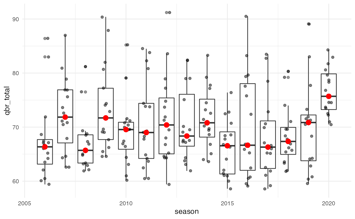
Alternatively you can also find the median by quarterback.
nfl_qbr_season %>%
  filter(qb_plays >= 100) %>%
  group_by(name_short) %>%
  summarize(
    median = median(qbr_total),
    years = range(season) %>% paste0(collapse = "-"),
    active = if_else(max(season) == 2020, "Active", "Retired"),
    .groups = "drop"
    ) %>%
  arrange(desc(median))
#> # A tibble: 135 × 4
#>    name_short  median years     active
#>    <chr>        <dbl> <chr>     <chr>
#>  1 P. Mahomes    80.6 2018-2020 Active
#>  2 P. Manning    76.9 2006-2015 Retired
#>  3 T. Brady      73.9 2006-2020 Active
#>  4 L. Jackson    73.7 2018-2020 Active
#>  5 Q. Gray       73.6 2007-2007 Retired
#>  6 D. Prescott   71.9 2016-2020 Active
#>  7 T. Collins    71.1 2007-2007 Retired
#>  8 D. Brees      70.8 2006-2020 Active
#>  9 D. Watson     70.5 2017-2020 Active
#> 10 A. Rodgers    69.6 2008-2020 Active
#> # … with 125 more rows