02 - Authoring Quarto
Quarto, anatomy
Metadata: YAML
Text: Markdown
Code:
knitrorjupyter
Add it all together, and you have beautiful, powerful, and useful outputs, all with plain text input!
Literate programming
Literate programming is writing out the program logic in a human language with included (separated by a primitive markup) code snippets and macros. - Wikipedia
---
title: "ggplot2 demo"
date: "5/22/2021"
format: html
---

## Air Quality

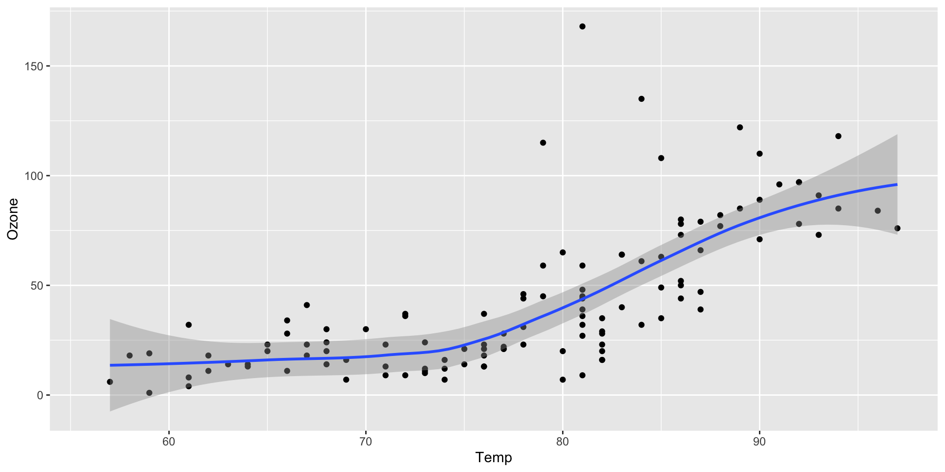
There is a relationship between temperature and the ozone level.

```{r}
#| label: fig-airquality
library(ggplot2)
ggplot(airquality, aes(Temp, Ozone)) +
  geom_point() +
  geom_smooth(method = "loess"
)
```
1 Metadata
Metadata: YAML
“Yet Another Markup Language” or “YAML Ain’t Markup Language”
Output Options
Why YAML?
To avoid manually typing out all the options, every time!
Demo: Navigating within RStudio
Quarto workflow
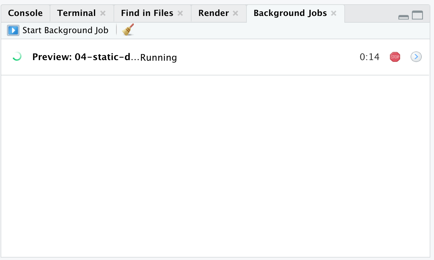
Executing the Quarto Render button in RStudio will call Quarto render in a background job - this will prevent Quarto rendering from cluttering up the R console, and gives you and easy way to stop.
Rendering
- Render in RStudio, starts a background job and previews the output

- System shell via
quarto render
- R console via
quartoR package
Our Turn
- Open RStudio and
quarto-workshop/03-computation/visual-editor.qmd - Compare behavior of rendering from RStudio > Render, using the CLI with
quarto render, and in R console viaquarto::quarto_render()
Quarto linting
Lint, or a linter, is a static code analysis tool used to flag programming errors, bugs, stylistic errors and suspicious constructs. - Lint


Quarto YAML Intelligence
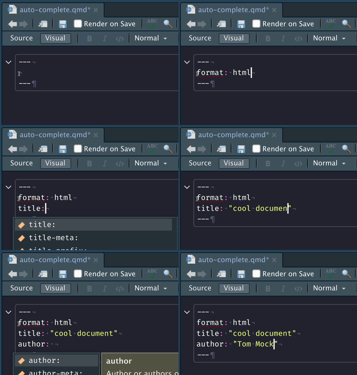
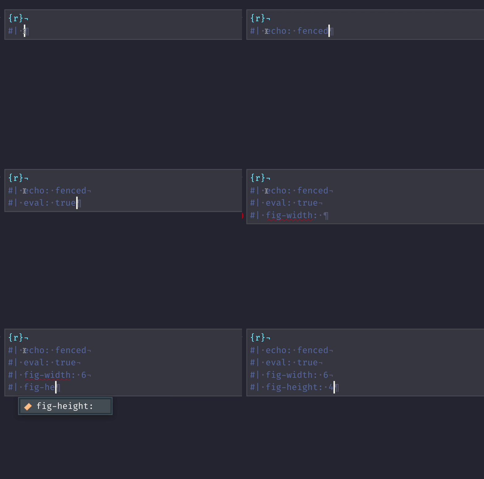
RStudio + VSCode provide rich tab-completion - start a word and tab to complete, or Ctrl + space to see all available options.
Single source publishing
Divs and Spans
Pandoc and therefore Quarto can parse “fenced Div blocks”
A paragraph with big text.
This is text with special formatting.
Divs and spans
A fenced div always starts and ends with equal/matching ::::
Why ::: instead of <div>
You’re not limited to HTML/CSS concepts - Pandoc and Quarto also have “attributes” that can be assigned in this way.
- You can think of a
:::div as a HTML<div>but it can also apply in specific situations to content in PDF or other formats (Word, Powerpoint, etc) - Similarly,
[text]{.class}spans can be thought of a<span .class>Text</span>but again are a bit more transferable if using Pandoc/Quarto native attributes.
The following, uses a ::: to apply a figure layout Quarto class across formats AND applies a span with {alt-text="text"}
Callout Blocks
:::{.callout-note}
Note that there are five types of callouts, including:
`note`, `tip`, `warning`, `caution`, and `important`.
:::
Note
Note that there are five types of callouts, including: note, tip, warning, caution, and important.
Warning
Callouts provide a simple way to attract attention, for example, to this warning.
This is important
Danger, callouts will really improve your writing.
Tip with caption
Caution, under construction
Here is something under construction
Callout markdown syntax
:::{.callout-note}
Note that there are five types of callouts, including:
`note`, `warning`, `important`, `tip`, and `caution`.
:::


:::{.callout-tip}
## Tip With Caption

This is an example of a callout with a caption.
:::
:::{.callout-caution collapse="true"}
## Expand To Learn About Collapse

This is an example of a 'folded' caution callout that can be expanded by the user. You can use `collapse="true"` to collapse it by default or `collapse="false"` to make a collapsible callout that is expanded by default.
:::
Our turn
- Open
quarto-workshop/02-authoring/callout-boxes.qmd - Try changing the types of callouts/remove them from code boxes and then render
- Open
quarto-workshop/02-authoring/callout-pdf.qmdand render it as well
Tabsets
Split up and flip between sections of a page, alternative to just two columns
::: {.panel-tabset}

## Element 1

## Element 2

:::
Tabsets
                   mpg cyl disp  hp drat    wt  qsec vs am gear carb
Mazda RX4         21.0   6  160 110 3.90 2.620 16.46  0  1    4    4
Mazda RX4 Wag     21.0   6  160 110 3.90 2.875 17.02  0  1    4    4
Datsun 710        22.8   4  108  93 3.85 2.320 18.61  1  1    4    1
Hornet 4 Drive    21.4   6  258 110 3.08 3.215 19.44  1  0    3    1
Hornet Sportabout 18.7   8  360 175 3.15 3.440 17.02  0  0    3    2
Valiant           18.1   6  225 105 2.76 3.460 20.22  1  0    3    1
Tabsets
Figure layout
- Use a
layoutdiv:::: {layout-ncol=2}or::: {layout-nrow=3}::: {layout="[[70,30], [100]]"}::: {layout="[[40,-20,40], [100]]"}
Figure Layout
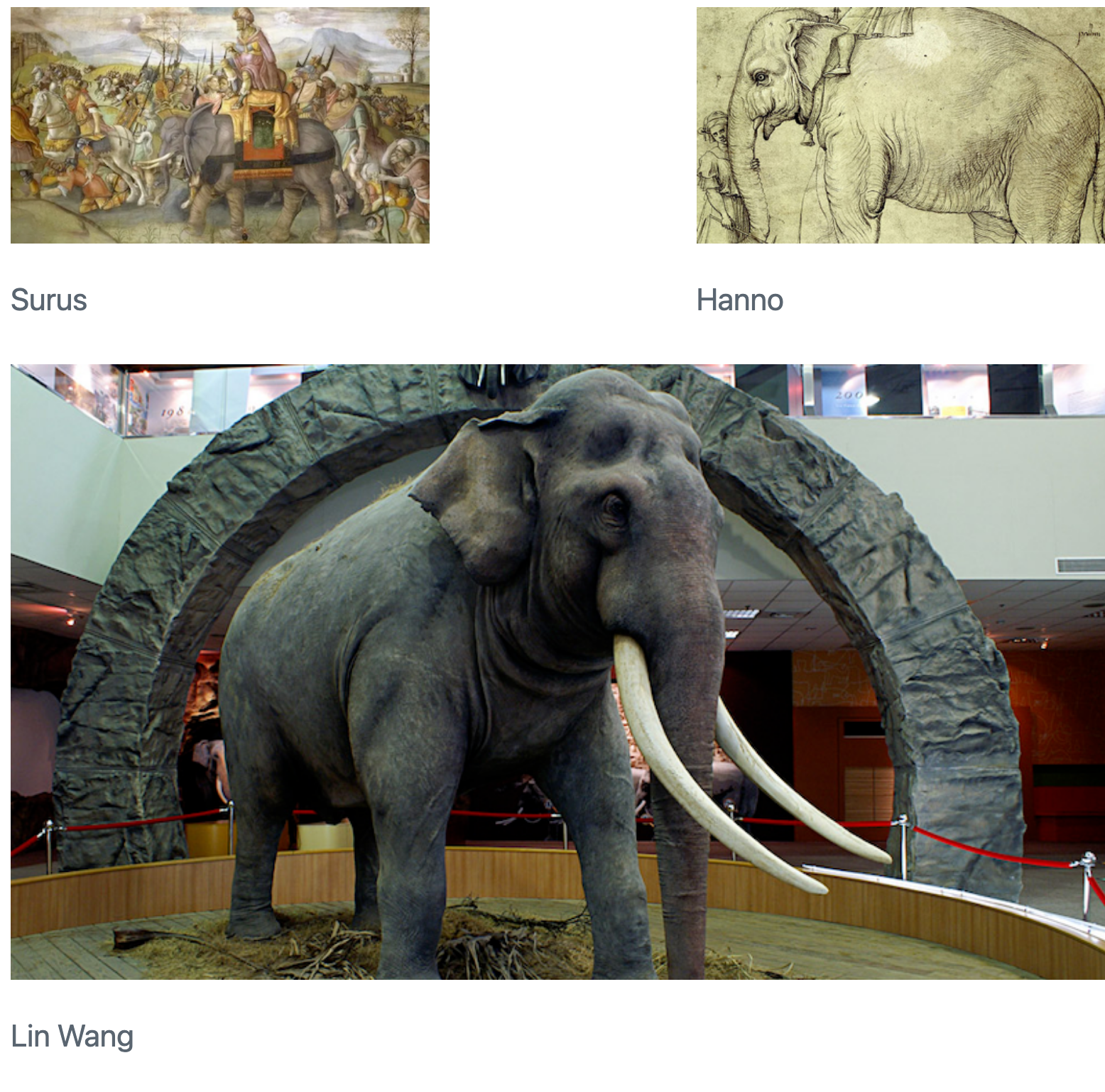
::: {layout="[[40,-20,40], [100]]"}


:::
Spans
Whereas a ::: fenced div is useful for application across a paragraph of text or set of images, a [span]{.class} is useful for application to a single item/string within a sentence.
Maybe a footnote1
Or a magically appearing word with an additional point after
Code
Choose your engine
If no engine specified, Quarto will use whatever language is found first (R = knitr, Python/Julia = Jupyter)
You can force using knitr if you’re mixing R/Python content via reticulate or if your first code chunk is not R but you want to use R.
knitr code cells
There’s a lot of knitr options!
- See Quarto specific
knitrdetails at: https://quarto.org/docs/reference/cells/cells-knitr.html knitroverview in total: https://yihui.org/knitr/- Jupyter specific chunk options: https://quarto.org/docs/reference/cells/cells-jupyter.html
Anatomy of a code chunk
Code
Code, more than just R
```{python}
#| label: fig-polar
#| eval: false
#| fig-cap: "A line plot on a polar axis"

import numpy as np
import matplotlib.pyplot as plt

r = np.arange(0, 2, 0.01)
theta = 2 * np.pi * r
fig, ax = plt.subplots(
  subplot_kw = {'projection': 'polar'}
)
ax.plot(theta, r)
ax.set_rticks([0.5, 1, 1.5, 2])
ax.grid(True)
plt.show()
```
Create code chunks
- You can manually type out code chunks:
```{r} - the keyboard shortcut
Ctrl + Alt + I(OS X:Cmd + Option + I) - the Add Chunk command in the editor toolbar
Or use the Command Palette: Cmd + Shift + P/Ctrl + Shift + P
Code chunks options
All code chunk options at yihui.org/knitr/options/
If you’ve used RMarkdown before, you’re likely used to syntax like:
```{r chunk-label, option=TRUE}
                mpg cyl  disp  hp drat    wt  qsec vs am gear carb
Fiat 128       32.4   4  78.7  66 4.08 2.200 19.47  1  1    4    1
Honda Civic    30.4   4  75.7  52 4.93 1.615 18.52  1  1    4    2
Toyota Corolla 33.9   4  71.1  65 4.22 1.835 19.90  1  1    4    1
Fiat X1-9      27.3   4  79.0  66 4.08 1.935 18.90  1  1    4    1
Porsche 914-2  26.0   4 120.3  91 4.43 2.140 16.70  0  1    5    2
Lotus Europa   30.4   4  95.1 113 3.77 1.513 16.90  1  1    5    2
Quarto introduces the “hash pipe” in #| - this is the preferred syntax, although Quarto is backwards compatible with the older RMarkdown syntax.
                mpg cyl  disp  hp drat    wt  qsec vs am gear carb
Fiat 128       32.4   4  78.7  66 4.08 2.200 19.47  1  1    4    1
Honda Civic    30.4   4  75.7  52 4.93 1.615 18.52  1  1    4    2
Toyota Corolla 33.9   4  71.1  65 4.22 1.835 19.90  1  1    4    1
Fiat X1-9      27.3   4  79.0  66 4.08 1.935 18.90  1  1    4    1
Porsche 914-2  26.0   4 120.3  91 4.43 2.140 16.70  0  1    5    2
Lotus Europa   30.4   4  95.1 113 3.77 1.513 16.90  1  1    5    2
Quarto’s hash pipe #|

Why Quarto + #|?
- Consistency across engine (Jupyter/knitr)
- Consistency across YAML/Chunk/
:::options - decrease mental burden when learning/remembering - More control over order/spacing of chunk options - not limited to one running line of options!
Quarto chunk options
```{r}
#| code-line-numbers: "|3-8"
#| warning: false
#| fig-cap: "Air Quality"
#| fig-align: left
#| fig-alt: |
#|   "A scatterplot with temperature by ozone levels along with a trend line
#|   indicating the increase in temperature with increasing ozone levels."

library(ggplot2)
ggplot(airquality, aes(Ozone, Temp)) +
        geom_point() +
        geom_smooth(method = "loess", se = FALSE)
```
Air Quality
Code in chunk option
You can also execute code inside a chunk option via the !expr syntax:
```{r}
#| code-line-numbers: "|3"
#| fig-cap: !expr glue::glue("The mean temperature was {mean(airquality$Temp) |> round()}")
#| fig-alt: |
#|   "A scatterplot with temperature by ozone levels along with a trend line
#|   indicating the increase in temperature with increasing ozone levels."
ggplot(airquality, aes(Ozone, Temp)) +
        geom_point() +
        geom_smooth(method = "loess", se = FALSE)
```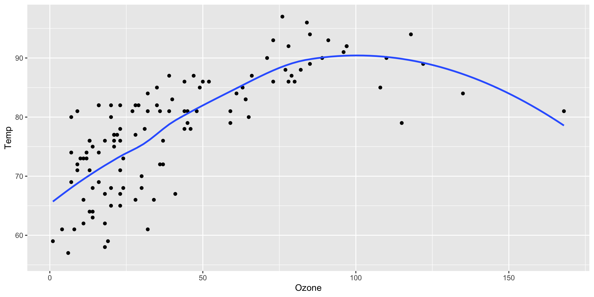
The mean temperature was 78
Quarto and RMarkdown
- Basic RMarkdown documents that render to static HTML and PDF are the most transferable directly to Quarto
Note that the YAML for Quarto:
- Will follow a
word-wordsyntax
- Instead of using
output: html_document, you’ll useformat: html
One source of the difference in syntax is that Quarto is more closely aligned with Pandoc format names and options (thus the use of - as a word separator rather than _).
Our turn
- Open
quarto-workshop/04-static/old-rmarkdown.rmd - Render via Quarto CLI
Converting RMarkdown -> Quarto
Option 1: Change
.rmd->.qmd- this will ALWAYS use Quarto for renderingOption 2: Change YAML’s
output: html_document->format: html- uses Quarto
Converting knitr chunks
knitrdev version as of 2022-08-06 has:knitr::convert_chunk_header("doc.qmd", output = identity)
knitr::convert_chunk_header()converts:fig.width=1syntax to#| fig-width: 1- across all code chunks in a entire document
But again - you don’t have to convert syntax of all your old documents, can use quarto render at terminal or use R + quarto::quarto_render() to render existing RMarkdown docs via Quarto
Remember the ::: {layout}?
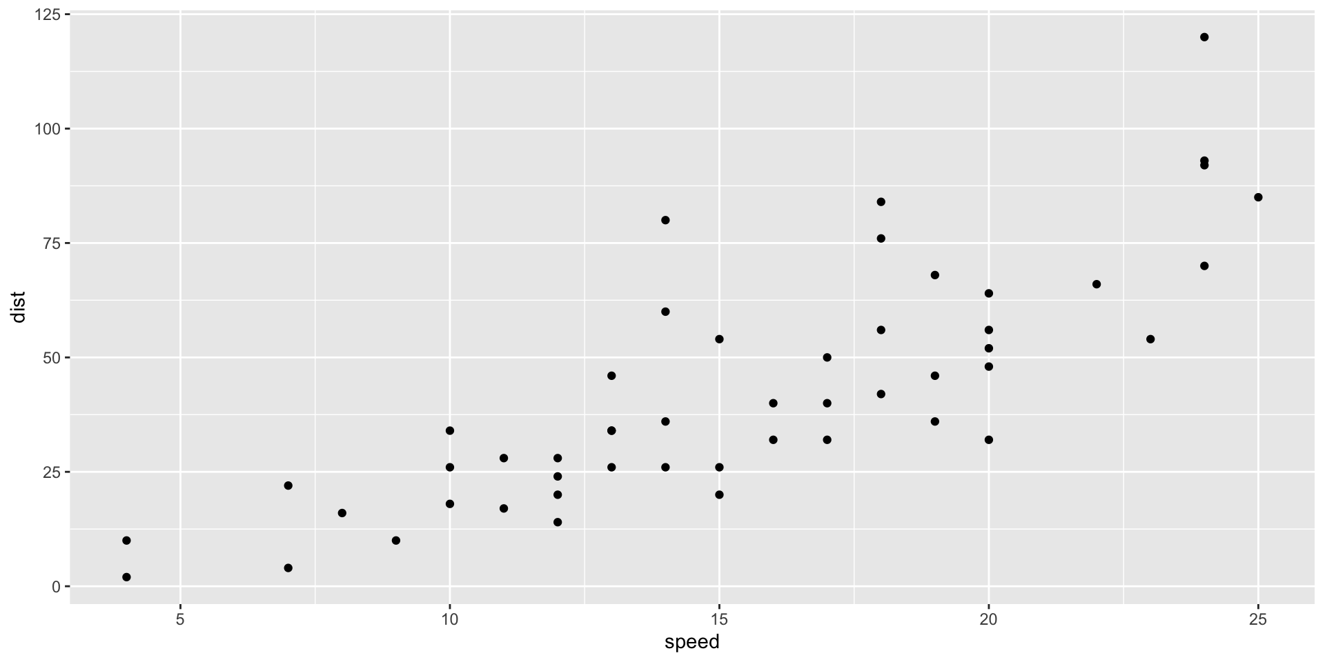
You can do similar things with chunk options and plots from code!
```{r}
#| code-line-numbers: "|4"
#| output-location: fragment
#| layout-ncol: 2
#| fig-cap:
#|   - "Speed and Stopping Distances of Cars"
#|   - "Engine displacement and fuel efficiency in Cars"
cars |>
  ggplot(aes(x = speed, y = dist)) +
  geom_point()
mtcars |>
  ggplot(aes(x = disp, y = mpg)) +
  geom_point()
```
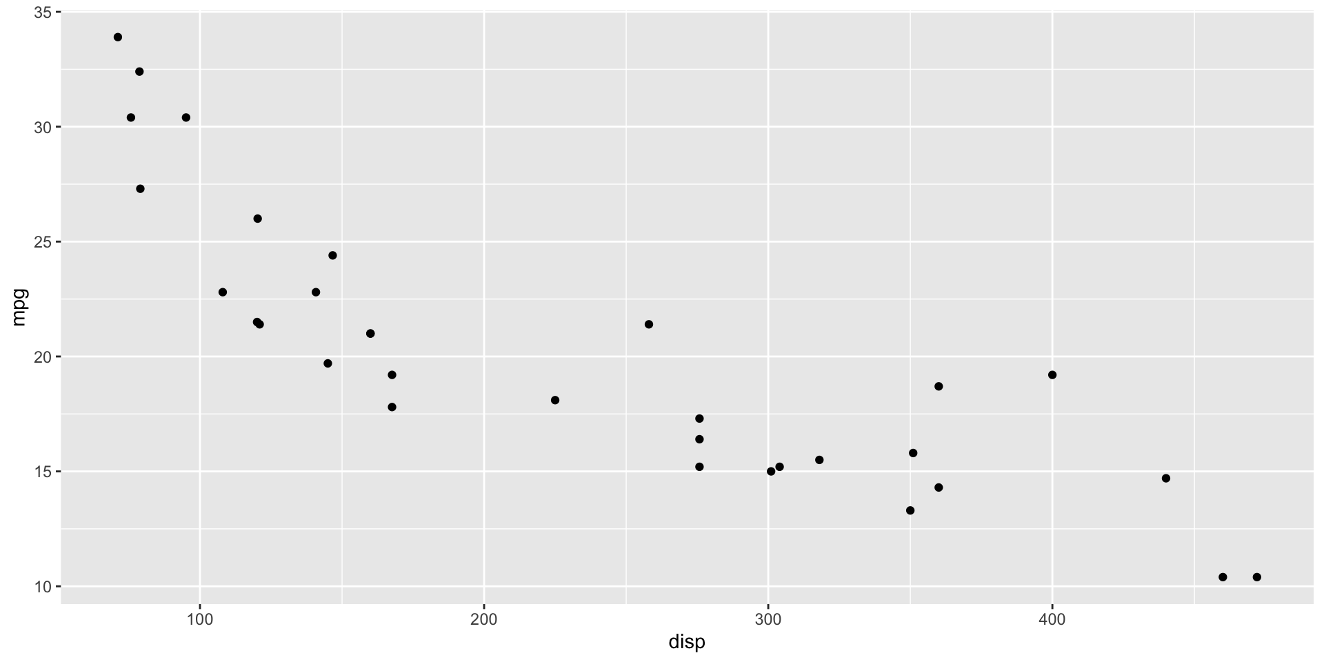
Chunk option layouts
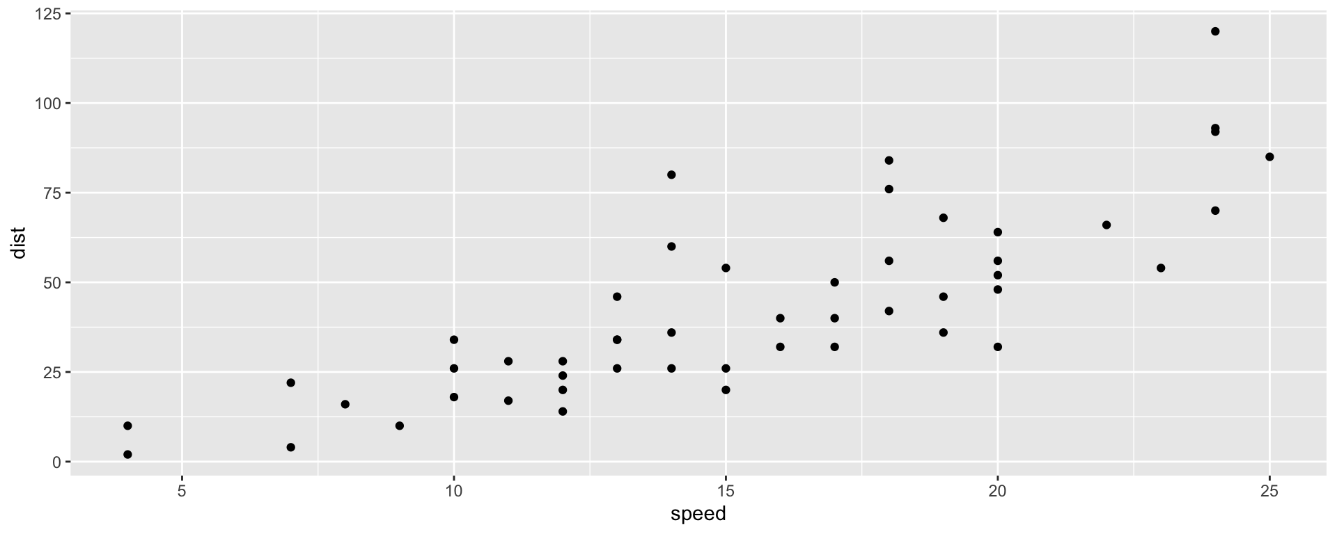
```{r}
#| code-line-numbers: "|7"
#| output-location: fragment
#| fig-cap:
#|   - "Speed and Stopping Distances of Cars"
#|   - "Engine displacement and fuel efficiency in Cars"
#| layout: "[[40,-20,40]]"
#| fig-height: 4
#| fig-format: retina
cars |>
  ggplot(aes(x = speed, y = dist)) +
  geom_point()
mtcars |>
  ggplot(aes(x = disp, y = mpg)) +
  geom_point()
```
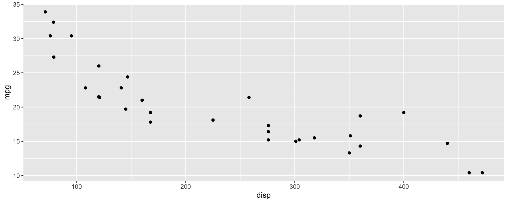
Aesthetics
HTML Appearance
Out of the box, Quarto’s HTML is styled with Bootstrap 5 and opinionated defaults.
Bootstrap is the most popular CSS Framework for responsive websites, where v5 is the latest.
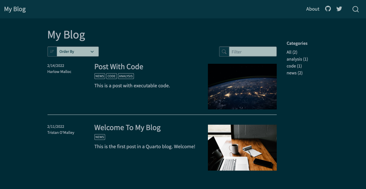
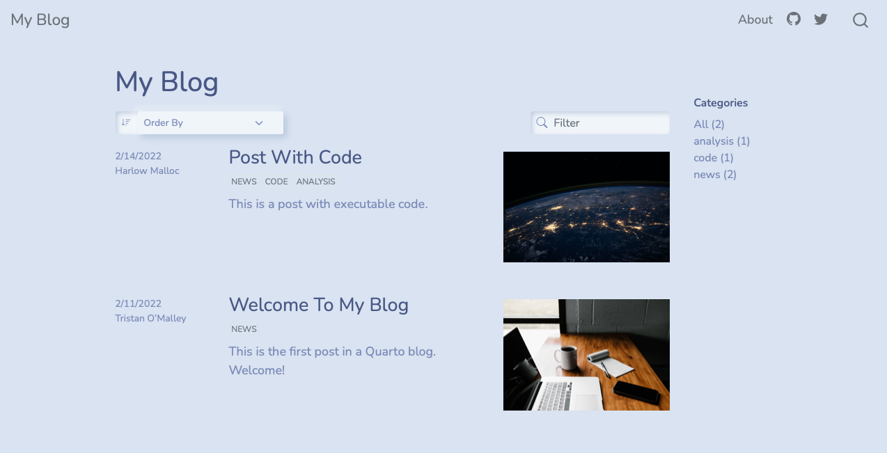
Quarto comes pre-installed with 25 themes from Bootswatch and you can use them like so:
Bootswatch themes
Our turn
- Open
quarto-workshop/04-static/bootswatch-themed.qmdand try out some themes!
- 25 bootswatch themes
Presentations
Embrace reveal.js
Embrace reveal.js
- Create new slides with level 1 or level 2 headers (
## Heading) - Add content/lists/images/code
Use fenced divs ::: for columns
- Content on the left
- More content
- Additional list
A paragraph of text that is important to hold on the left, but it’s fun to include below a list.
- Image on the right

Columns
Quarto Projects
Quarto projects
Quarto projects are directories that provide:
A way to render all or some of the files in a directory with a single command (e.g. quarto render myproject).
A way to share YAML configuration across multiple documents.
The ability to redirect output artifacts to another directory.
The ability to freeze rendered output (i.e. don’t re-execute documents unless they have changed).
In addition, projects can have special “types” that introduce additional behavior (e.g. websites or books).
Quarto Projects
- A Quarto Project is at minimal one Quarto document and the
_quarto.ymlfile
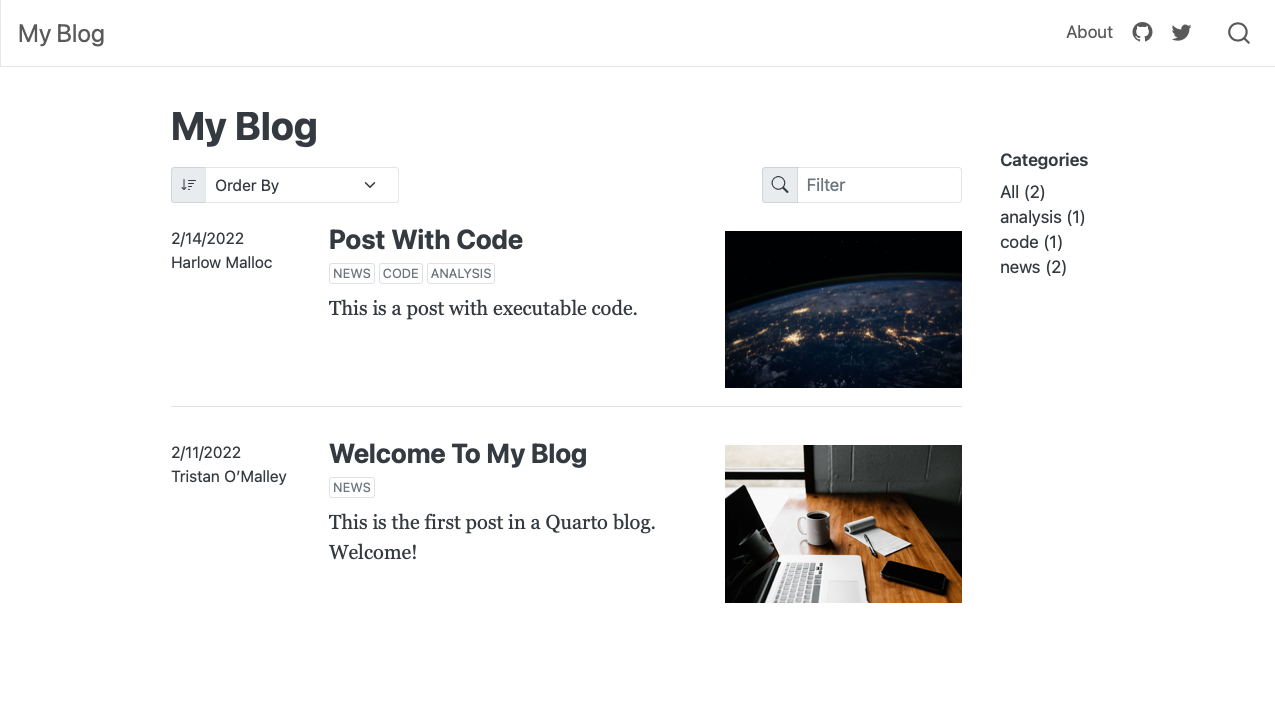
Quarto Projects
- Books, Websites, Blogs are a Quarto project
- Want to learn how to build a blog? Join Isabella Velasquez from RStudio in our next Quarto webinar!
- Add to your calendar: rstd.io/quarto-blog
Quarto, crafted with love and care
Development of Quarto is sponsored by RStudio, PBC. The same core team works on both Quarto and R Markdown:
Carlos Scheidegger (@cscheid)
Charles Teague (@dragonstyle)
Christophe Dervieux (@cderv)
J.J. Allaire (@jjallaire)
Yihui Xie (@yihui)
Here is the full contributors list. Quarto is open source and we welcome contributions in our github repository as well! https://github.com/quarto-dev/quarto-cli.
Quarto
- Batteries included, shared syntax across output types and languages
- Choose your own editor and your preferred data science language
- RMarkdown still maintained, but majority of new features built into Quarto
Follow @quarto_pub or me @thomas_mock on Twitter to stay up to date!
- Webinar Slides: https://jthomasmock.github.io/quarto-2hr-webinar/
- FULL workshop materials: rstd.io/get-started-quarto
- Workshop materials on RStudio Cloud:https://rstudio.cloud/content/4332583
Web resources
- Quarto.org for documentation or the Quarto FAQ
- “With Quarto Coming, is R Markdown Going Away? No.” - Yihui.org
Why the name “Quarto”?1
