Quarto workflow
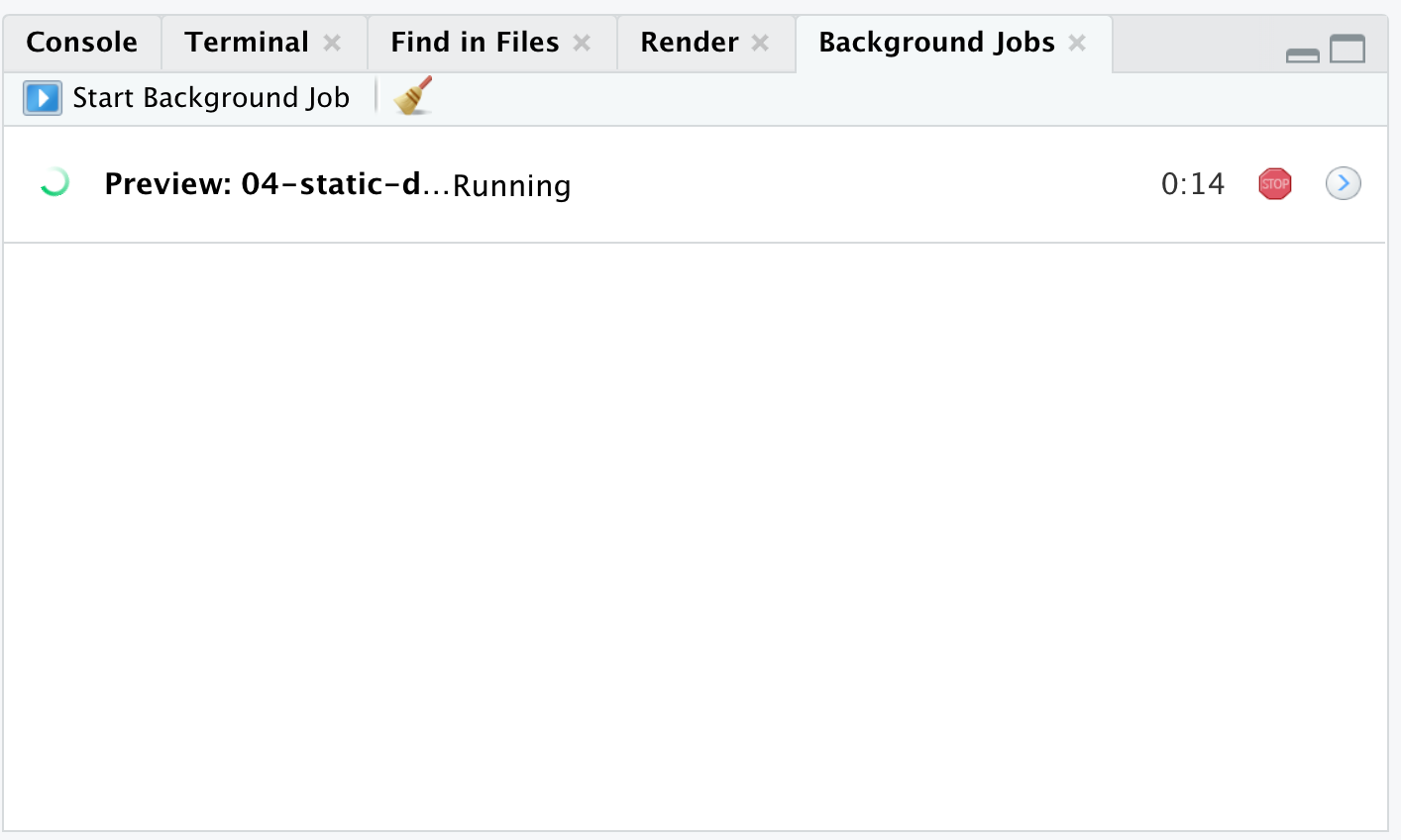
Executing the Quarto Render button in RStudio will call Quarto render in a background job - this will prevent Quarto rendering from cluttering up the R console, and gives you and easy way to stop.
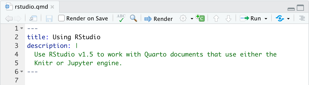
Rendering
- Render in RStudio, starts a background job and previews the output
- System shell via
quarto render
- R console via
quartoR package
Quarto linting
Lint, or a linter, is a static code analysis tool used to flag programming errors, bugs, stylistic errors and suspicious constructs. - Lint
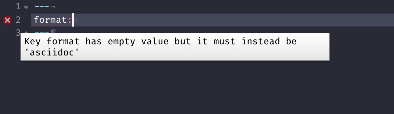
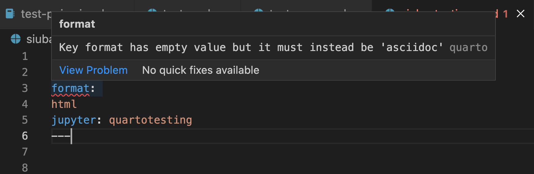
Quarto YAML Intelligence
RStudio + VSCode provide rich tab-completion - start a word and tab to complete, or Ctrl + space to see all available options.
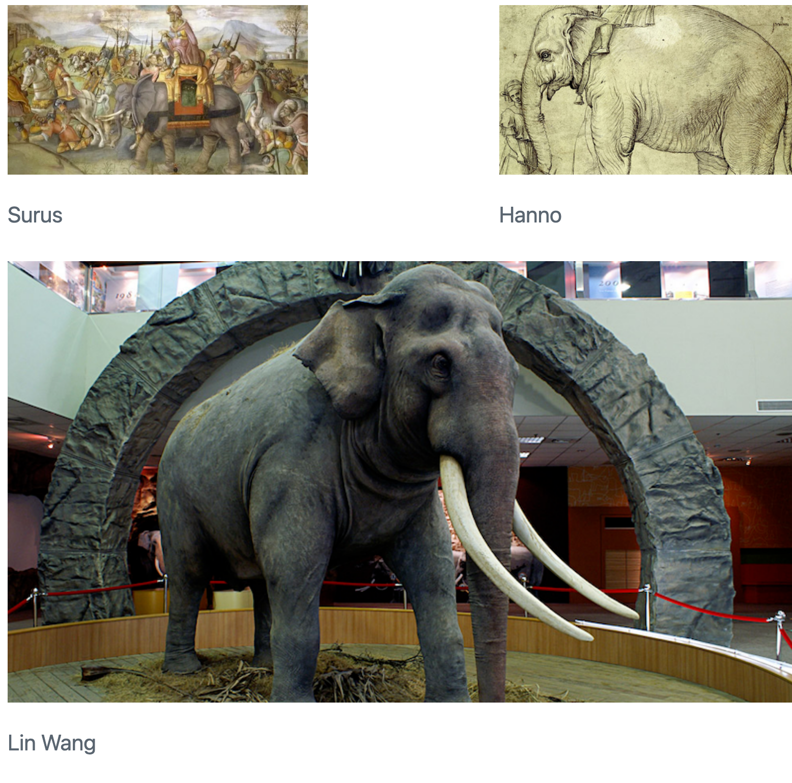
Figure Layout
::: {layout="[[40,-20,40], [100]]"}


:::
Code
Code, more than just R
```{python}
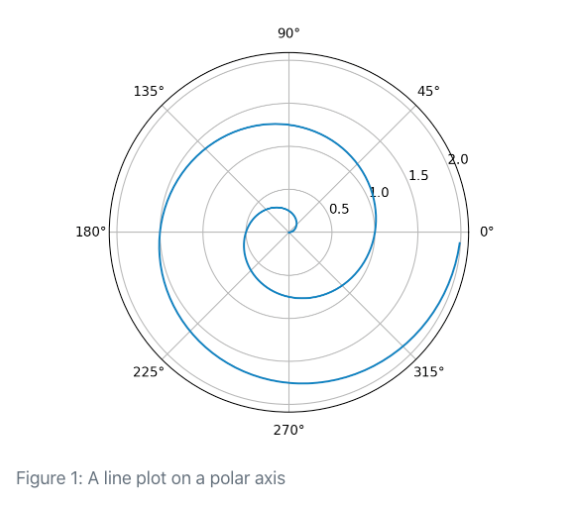
#| label: fig-polar
#| eval: false
#| fig-cap: "A line plot on a polar axis"
import numpy as np
import matplotlib.pyplot as plt
r = np.arange(0, 2, 0.01)
theta = 2 * np.pi * r
fig, ax = plt.subplots(
subplot_kw = {'projection': 'polar'}
)
ax.plot(theta, r)
ax.set_rticks([0.5, 1, 1.5, 2])
ax.grid(True)
plt.show()
```
Quarto’s hash pipe #|

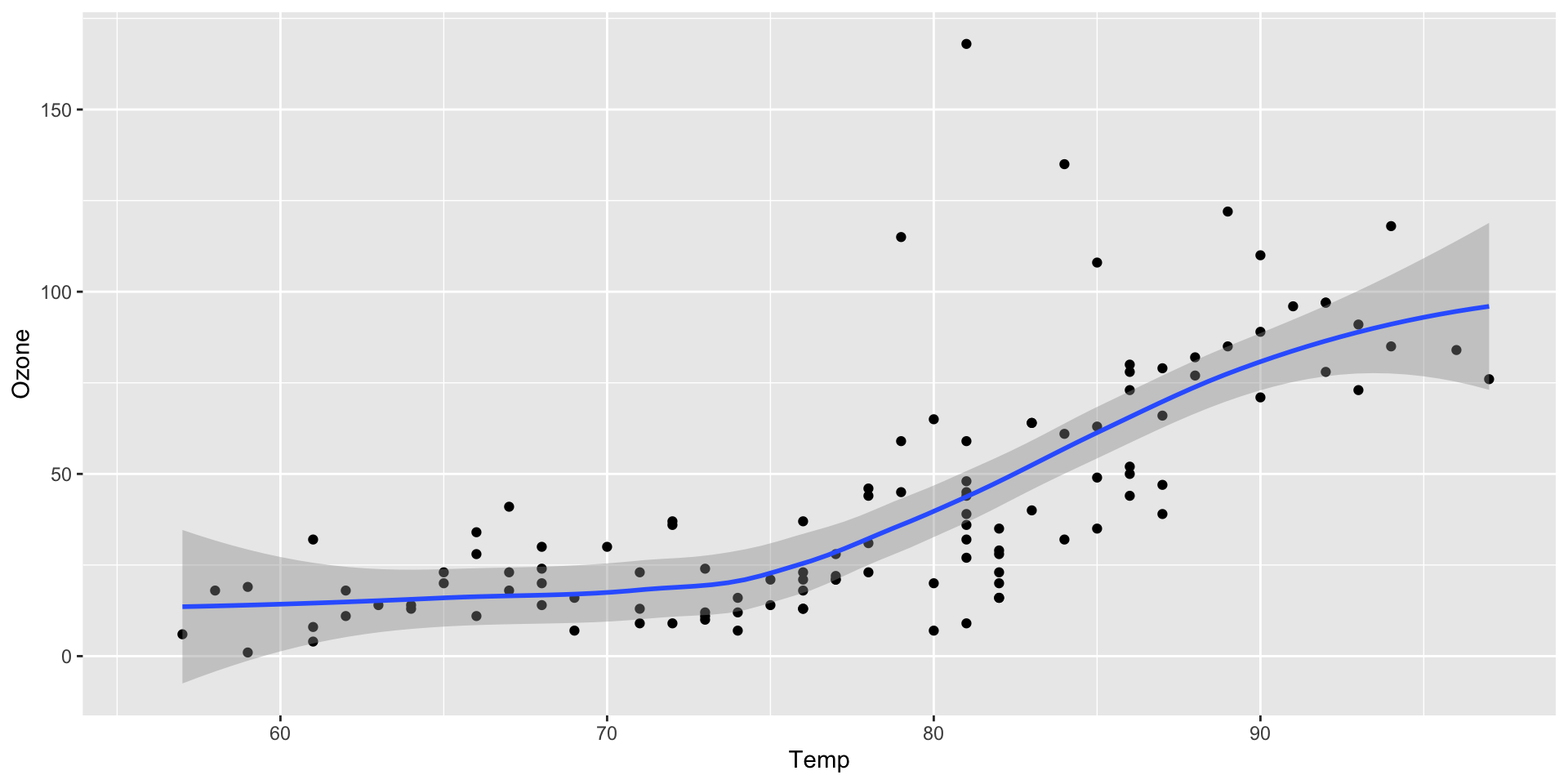
Quarto chunk options
```{r}
#| code-line-numbers: "|3-8"
#| warning: false
#| fig-cap: "Air Quality"
#| fig-align: left
#| fig-alt: |
#|   "A scatterplot with temperature by ozone levels along with a trend line
#|   indicating the increase in temperature with increasing ozone levels."

library(ggplot2)
ggplot(airquality, aes(Ozone, Temp)) +
        geom_point() +
        geom_smooth(method = "loess", se = FALSE)
```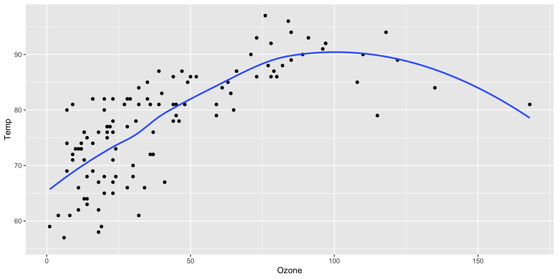
Air Quality
Code in chunk option
You can also execute code inside a chunk option via the !expr syntax:
```{r}
#| code-line-numbers: "|3"
#| fig-cap: !expr glue::glue("The mean temperature was {mean(airquality$Temp) |> round()}")
#| fig-alt: |
#|   "A scatterplot with temperature by ozone levels along with a trend line
#|   indicating the increase in temperature with increasing ozone levels."
ggplot(airquality, aes(Ozone, Temp)) +
        geom_point() +
        geom_smooth(method = "loess", se = FALSE)
```
The mean temperature was 78
Remember the ::: {layout}?
You can do similar things with chunk options and plots from code!
```{r}
#| code-line-numbers: "|4"
#| output-location: fragment
#| layout-ncol: 2
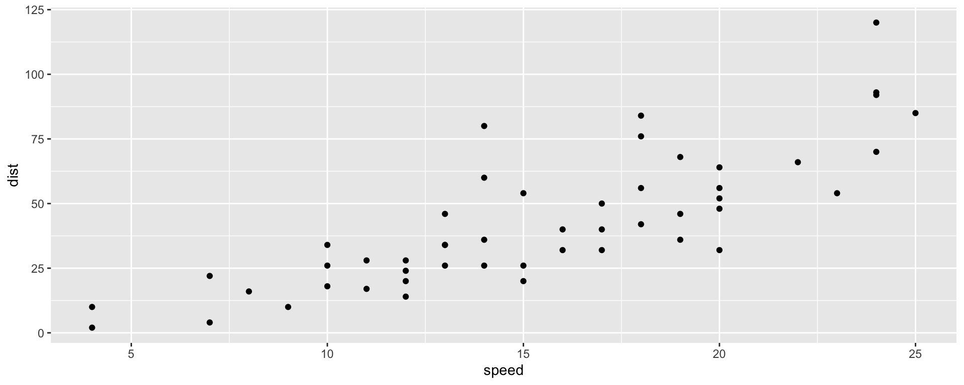
#| fig-cap:
#| - "Speed and Stopping Distances of Cars"
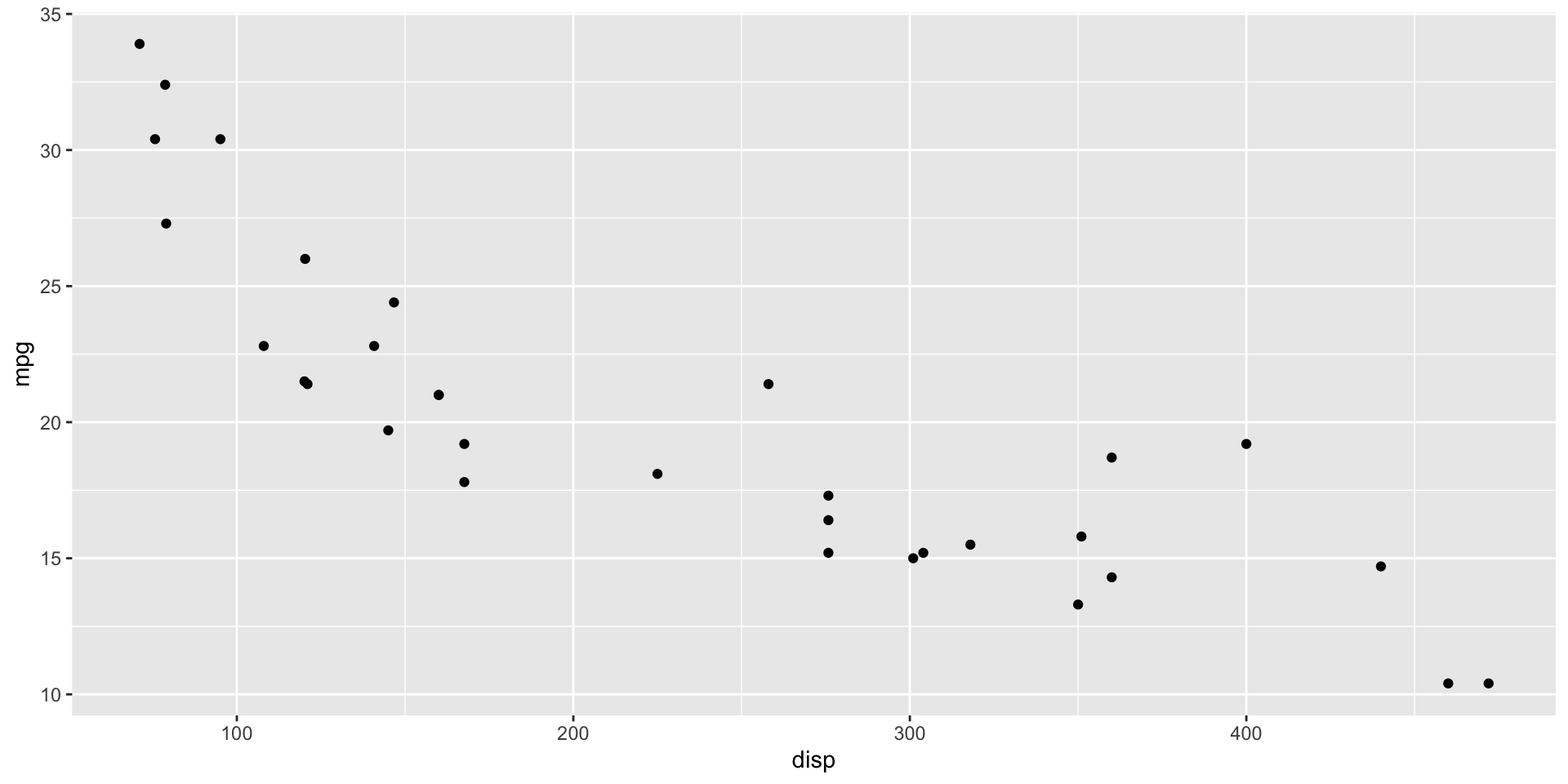
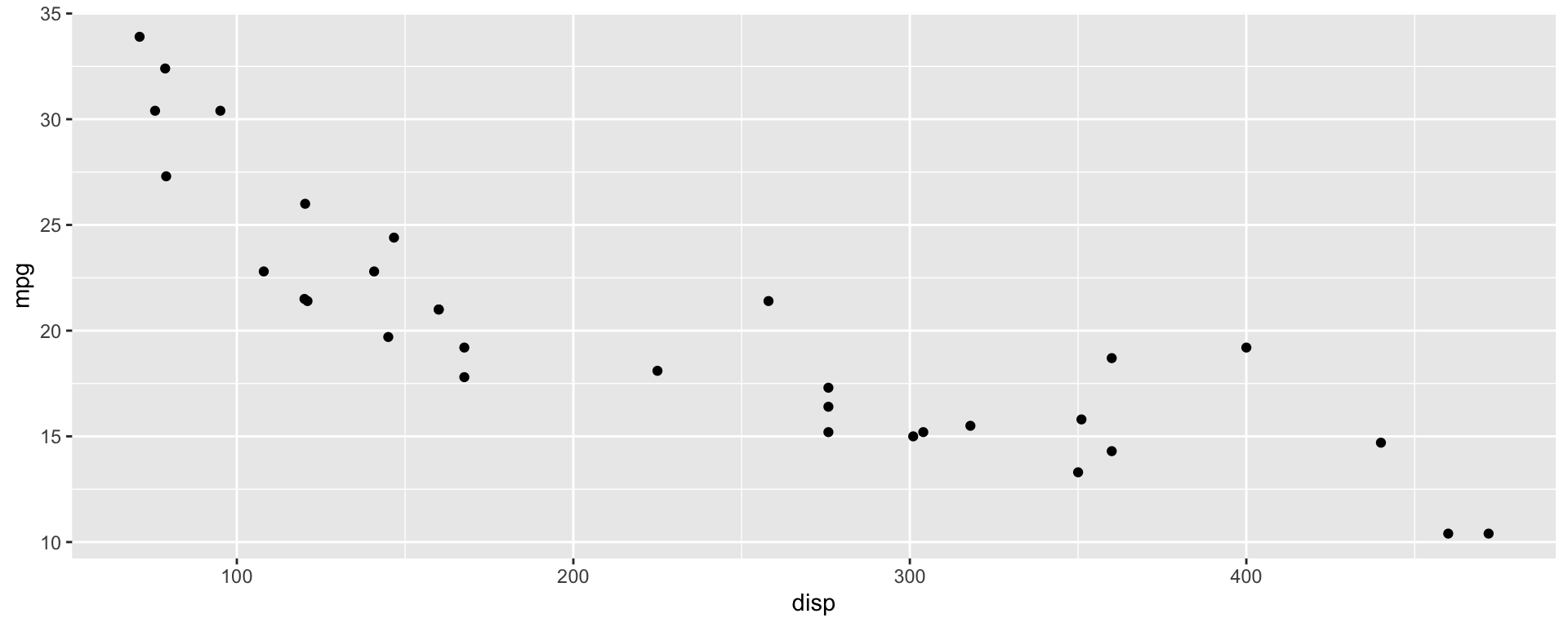
#| - "Engine displacement and fuel efficiency in Cars"
cars |>
ggplot(aes(x = speed, y = dist)) +
geom_point()
mtcars |>
ggplot(aes(x = disp, y = mpg)) +
geom_point()
```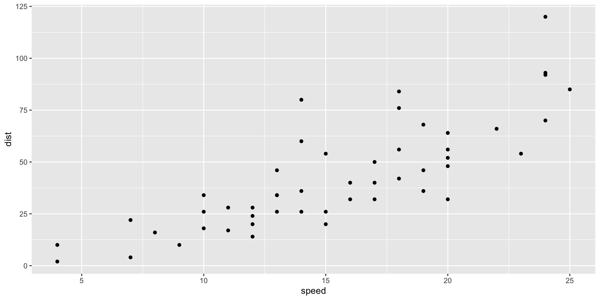
Chunk option layouts
```{r}
#| code-line-numbers: "|7"
#| output-location: fragment
#| fig-cap:
#|   - "Speed and Stopping Distances of Cars"
#|   - "Engine displacement and fuel efficiency in Cars"
#| layout: "[[40,-20,40]]"
#| fig-height: 4
#| fig-format: retina
cars |>
  ggplot(aes(x = speed, y = dist)) +
  geom_point()
mtcars |>
  ggplot(aes(x = disp, y = mpg)) +
  geom_point()
```
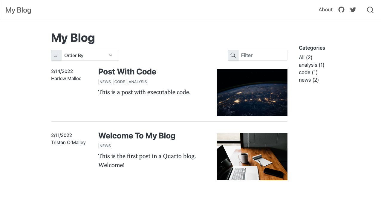
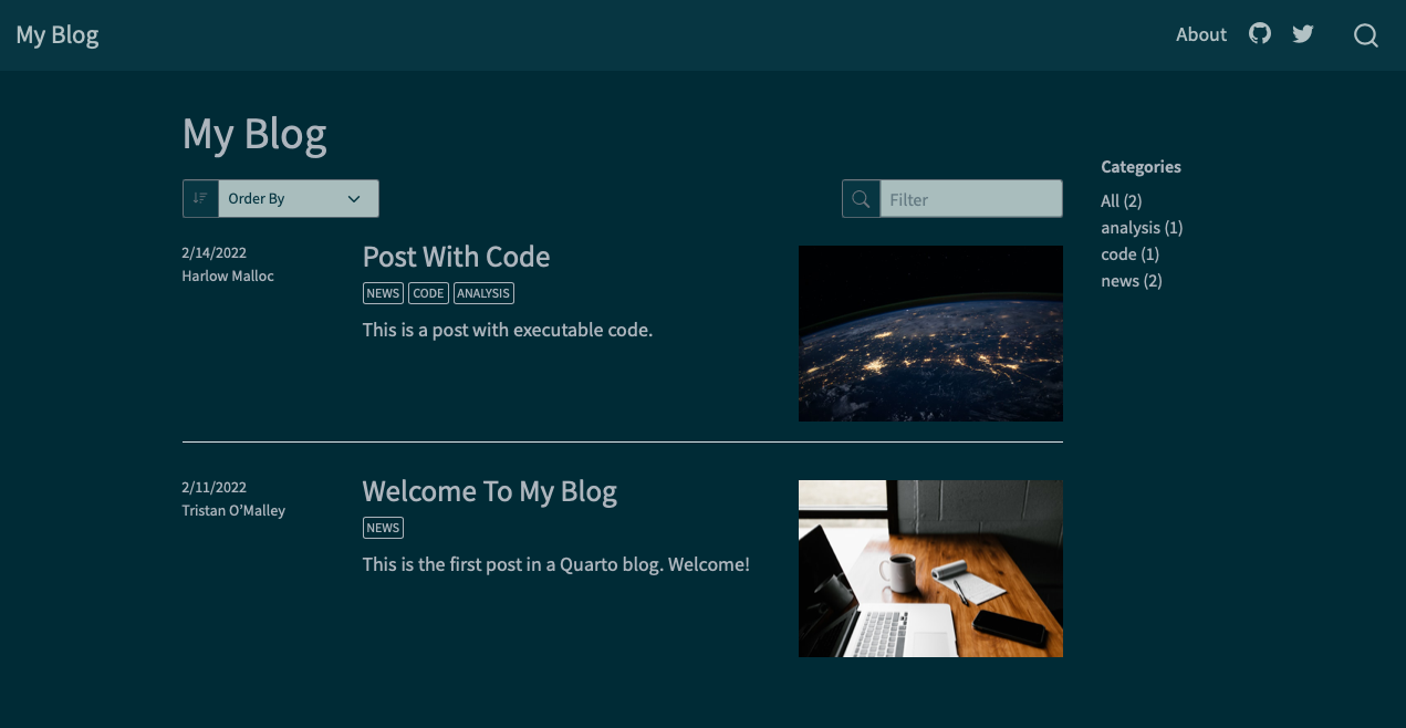
Bootswatch themes
Embrace reveal.js
- Create new slides with level 1 or level 2 headers (
## Heading) - Add content/lists/images/code
Use fenced divs ::: for columns
- Content on the left
- More content
- Additional list
A paragraph of text that is important to hold on the left, but it’s fun to include below a list.
- Image on the right

Why the name “Quarto”?1


![]()